Algorithm For Loss Function and introduction

Common Loss functions in machine learning-

1)Regression losses and 

2)Classification losses.

  There are three types of Regression losses

1.Mean Square Error/Quadratic Loss/L2 Loss

Mathematical formulation:

Algorithm-

import numpy as npy_hat = np.array([0.000, 0.166, 0.333])
y_true = np.array([0.000, 0.254, 0.998])def rmse(predictions, targets):
    differences = predictions - targets
    differences_squared = differences ** 2
    mean_of_differences_squared = differences_squared.mean()
    rmse_val = np.sqrt(mean_of_differences_squared)
    return rmse_valprint("d is: " + str(["%.8f" % elem for elem in y_hat]))
print("p is: " + str(["%.8f" % elem for elem in y_true]))rmse_val = rmse(y_hat, y_true)
print("rms error is: " + str(rmse_val))

2.Mean Absolute Error/L1 Loss

Mathematical formulation:-

Algorithm-

import numpy as npy_hat = np.array([0.000, 0.166, 0.333])
y_true = np.array([0.000, 0.254, 0.998])

print("d is: " + str(["%.8f" % elem for elem in y_hat]))
print("p is: " + str(["%.8f" % elem for elem in y_true]))

def mae(predictions, targets):
    differences = predictions - targets
    absolute_differences = np.absolute(differences)
    mean_absolute_differences = absolute_differences.mean()
    return mean_absolute_differencesmae_val = mae(y_hat, y_true)
print ("mae error is: " + str(mae_val))

3.Mean Bias Error

Mathematical formulation:-

This is much less common in the machine learning domain as compared to its counterpart. This is the same as MSE with the only difference that we don’t take absolute values. Clearly, there’s a need for caution as positive and negative errors could cancel each other out. Although less accurate in practice, it could determine if the model has a positive bias or negative bias.

Classification losses.

There are two types of Classification losses.

1.Hinge Loss/Multi class SVM Loss

In simple terms, the score of correct category should be greater than sum of scores of all incorrect categories by some safety margin (usually one). And hence hinge loss is used for maximum-margin classification, most notably for support vector machines. Although not differentiable, it’s a convex function which makes it easy to work with usual convex optimizers used in machine learning domain.

Mathematical formulation :-

SVM Loss or Hinge Loss

Consider an example where we have three training examples and three classes to predict — Dog, cat and horse. Below the values predicted by our algorithm for each of the classes :-

Hinge loss/ Multi class SVM loss

Computing hinge losses for all 3 training examples :-

## 1st training example
max(0, (1.49) - (-0.39) + 1) + max(0, (4.21) - (-0.39) + 1)
max(0, 2.88) + max(0, 5.6)
2.88 + 5.6
8.48 (High loss as very wrong prediction)## 2nd training example
max(0, (-4.61) - (3.28)+ 1) + max(0, (1.46) - (3.28)+ 1)
max(0, -6.89) + max(0, -0.82)
0 + 0
0 (Zero loss as correct prediction)## 3rd training example
max(0, (1.03) - (-2.27)+ 1) + max(0, (-2.37) - (-2.27)+ 1)
max(0, 4.3) + max(0, 0.9)
4.3 + 0.9
5.2 (High loss as very wrong prediction)

2.Cross-Entropy Loss/Negative Log-Likelihood

This is the most common setting for classification problems. Cross-entropy loss increases as the predicted probability diverge from the actual label.

Mathematical formulation:-

Cross entropy loss

Notice that when actual label is 1 (y(i) = 1), second half of function disappears whereas in case actual label is 0 (y(i) = 0) first half is dropped off. In short, we are just multiplying the log of the actual predicted probability for the ground truth class. An important aspect of this is that cross entropy loss penalizes heavily the predictions that are confident but wrong.

import numpy as nppredictions = np.array([[0.25,0.25,0.25,0.25],
                        [0.01,0.01,0.01,0.96]])
targets = np.array([[0,0,0,1],
                   [0,0,0,1]])def cross_entropy(predictions, targets, epsilon=1e-10):
    predictions = np.clip(predictions, epsilon, 1. - epsilon)
    N = predictions.shape[0]
    ce_loss = -np.sum(np.sum(targets * np.log(predictions + 1e-5)))/N
    return ce_losscross_entropy_loss = cross_entropy(predictions, targets)
print ("Cross entropy loss is: " + str(cross_entropy_loss))

Introduction to Loss Functions

The loss function is the bread and butter of modern machine learning; it takes your algorithm from theoretical to practical and transforms neural networks from glorified matrix multiplication into deep learning.

This post will explain the role of loss functions and how they work, while surveying a few of the most popular from the past decade.

---

What’s a Loss Function?

At its core, a loss function is incredibly simple: it’s a method of evaluating how well your algorithm models your dataset. If your predictions are totally off, your loss function will output a higher number. If they’re pretty good, it’ll output a lower number. As you change pieces of your algorithm to try and improve your model, your loss function will tell you if you’re getting anywhere.

In fact, we can design our own (very) basic loss function to further explain how it works. For each prediction that we make, our loss function will simply measure the absolute difference between our prediction and the actual value. In mathematical notation, it might look something like abs(y_predicted – y). Here’s what some situations might look like if we were trying to predict how expensive the rent is in some NYC apartments:

Notice how in the loss function we defined, it doesn’t matter if our predictions were too high or too low. All that matters is how incorrect we were, directionally agnostic. This is not a feature of all loss functions: in fact, your loss function will vary significantly based on the domain and unique context of the problem that you’re applying machine learning to. In your project, it may be much worse to guess too high than to guess too low, and the loss function you select must reflect that.

Different Types and Flavors of Loss Functions

A lot of the loss functions that you see implemented in machine learning can get complex and confusing. Consider this paper from late 2017, entitled A Semantic Loss Function for Deep Learning with Symbolic Knowledge. There’s more in that title that I don’t understand than I do. But if you remember the end goal of all loss functions–measuring how well your algorithm is doing on your dataset–you can keep that complexity in check.

We’ll run through a few of the most popular loss functions currently being used, from simple to more complex.

Mean Squared Error

Mean Squared Error (MSE) is the workhorse of basic loss functions: it’s easy to understand and implement and generally works pretty well. To calculate MSE, you take the difference between your predictions and the ground truth, square it, and average it out across the whole dataset.

Implemented in code, MSE might look something like:

def MSE(y_predicted, y):

squared_error = (y_predicted - y) ** 2

sum_squared_error = np.sum(squared_error)

mse = sum_squared_error / y.size

return(mse)

Likelihood Loss

The likelihood function is also relatively simple, and is commonly used in classification problems. The function takes the predicted probability for each input example and multiplies them. And although the output isn’t exactly human interpretable, it’s useful for comparing models.

For example, consider a model that outputs probabilities of [0.4, 0.6, 0.9, 0.1] for the ground truth labels of [0, 1, 1, 0]. The likelihood loss would be computed as (0.6) * (0.6) * (0.9) * (0.9) = 0.2916. Since the model outputs probabilities for TRUE (or 1) only, when the ground truth label is 0 we take (1-p) as the probability. In other words, we multiply the model’s outputted probabilities together for the actual outcomes.

Log Loss (Cross Entropy Loss)

Log Loss is a loss function also used frequently in classification problems, and is one of the most popular measures for Kaggle competitions. It’s just a straightforward modification of the likelihood function with logarithms.

This is actually exactly the same formula as the regular likelihood function, but with logarithms added in. You can see that when the actual class is 1, the second half of the function disappears, and when the actual class is 0, the first half drops. That way, we just end up multiplying the log of the actual predicted probability for the ground truth class.

The cool thing about the log loss loss function is that is has a kick: it penalizes heavily for being very confident and very wrong. Predicting high probabilities for the wrong class makes the function go crazy. The graph below is for when the true label =1, and you can see that it skyrockets as the predicted probability for label = 0 approaches 1.

Loss Functions and Optimizers

Loss functions provide more than just a static representation of how your model is performing–they’re how your algorithms fit data in the first place. Most machine learning algorithms use some sort of loss function in the process of optimization or finding the best parameters (weights) for your data.

For a simple example, consider linear regression. In traditional “least squares” regression, the line of best fit is determined through none other than MSE (hence the least-squares moniker)! For each set of weights that the model tries, the MSE is calculated across all input examples. The model then optimizes the MSE functions––or in other words, makes it the lowest possible––through the use of an optimizer algorithm like Gradient Descent.

Just like there are different flavors of loss functions for unique problems, there is no shortage of different optimizers as well. That’s beyond the scope of this post, but in essence, the loss function and optimizer work in tandem to fit the algorithm to your data in the best way possible.

MDP Algorithm (Markov decision process)

-- |
-- Module     : Algorithms.MDP
-- Copyright  : Patrick Steele 2015
-- License    : MIT (see the LICENSE file)
-- Maintainer : prs233@cornell.edu
--
-- Algorithms and data structures for expressing and solving Markov
-- decision processes (MDPs).
--
-- See the following for references on the algorithms implemented,
-- along with general terminology.
--
-- * \"Dynamic Programmand and Optimal Control, Vol. II\", by Dimitri
--   P. Bertsekas, Athena Scientific, Belmont, Massachusetts.
--
-- * \"Stochastic Dynamic Programming and the Control of Queueing
--   Systems\", by Linn I. Sennott, A Wiley- Interscience Publication,
--   New York.
--
-- The module "Algorithms.MDP.Examples" contains implementations of
-- several example problems from these texts.
--
-- To actually solve an MDP, use (for example) the
-- 'Algorithms.MDP.ValueIteration.valueIteration' function from the
-- "Algorithms.MDP.ValueIteration" module.
module Algorithms.MDP
       ( -- * Markov decision processes
         MDP (..)
       , mkDiscountedMDP
       , mkUndiscountedMDP
         -- * Types
       , Transitions
       , Costs
       , ActionSet
       , CF
       , CFBounds (..)
         -- * Utility functions
       , cost
       , action
       , optimalityGap
         -- * Validation
       , verifyStochastic
       , MDPError (..)
       ) where

import qualified Data.Vector as V
import Data.Maybe

-- | A type representing an action- and state-dependent probablity
-- vector.
type Transitions a b t = b -> a -> a -> t

-- | A type representing an action- and state-dependent cost.
type Costs a b t = b -> a -> t

-- | A type representing the allowed actions in a state.
type ActionSet a b = a -> [b]

-- | A cost function is a vector containing (state, action, cost)
-- triples. Each triple describes the cost of taking the action in
-- that state.
type CF a b t = V.Vector (a, b, t)

-- | Get the cost associated with a state.
--
-- This function is only defined over the state values passed in to
-- the original MDP.
cost :: (Eq a) => a -> CF a b t -> t
cost s cf = 
  let
    (_, _, c) = fromMaybe err (V.find (\(s', _, _) -> s == s') cf)
    err = error "Unknown state in function \"cost\""
  in
    c

-- | Get the action associated with a state.
--
-- This function is only defined over the state values passed in to
-- the original MDP.
action :: (Eq a) => a -> CF a b t -> b
action s cf =
  let
    (_, ac, _) = fromMaybe err (V.find (\(s', _, _) -> s == s') cf)
    err = error "Unknown state in function \"action\""
  in
    ac

-- | A cost function with error bounds. The cost in a (state, action,
-- cost) triple is guaranteed to be in the range [cost + lb, cost + ub]
data CFBounds a b t = CFBounds
                      { _CF :: CF a b t
                      , _lb :: t
                      , _ub :: t
                      }

-- | Compute the optimality gap associated with a CFBounds.
--
-- This error is absolute, not relative.
optimalityGap :: (Num t) => CFBounds a b t -> t
optimalityGap (CFBounds _ lb ub) = ub - lb

-- | A Markov decision process.
--
-- An MDP consists of a state space, an action space, state- and
-- action-dependent costs, and state- and action-dependent transition
-- probabilities. The goal is to compute a policy -- a mapping from
-- states to actions -- which minimizes the total discounted cost of
-- the problem, assuming a given discount factor in the range (0, 1].
--
-- Here the type variable 'a' represents the type of the states, 'b'
-- represents the type of the actions, and 't' represents the numeric
-- type used in computations. Generally choosing 't' to be a Double is
-- fine, although there is no reason a higher-precision type cannot be
-- used.
--
-- This type should not be constructed directly; use the
-- 'mkDiscountedMDP' or 'mkUndiscountedMDP' constructors instead.
data MDP a b t = MDP
                 { _states    :: V.Vector a
                 , _actions   :: V.Vector b
                 , _costs     :: V.Vector (V.Vector t)
                 , _trans     :: V.Vector (V.Vector (V.Vector t))
                 , _discount  :: t
                 , _actionSet :: V.Vector (V.Vector Int)
                 }

-- | Creates a discounted MDP.
mkDiscountedMDP :: (Eq b) =>
             [a]                -- ^ The state space
          -> [b]                -- ^ The action space
          -> Transitions a b t  -- ^ The transition probabilities
          -> Costs a b t        -- ^ The action-dependent costs
          -> ActionSet a b      -- ^ The state-dependent actions
          -> t                  -- ^ The discount factor
          -> MDP a b t          -- ^ The resulting DiscountedMDP
mkDiscountedMDP states actions trans costs actionSet discount =
  let
    _states      = V.fromList states
    _actions     = V.fromList actions
    mkProbAS a s = V.fromList $ map (trans a s) states
    mkProbA a    = V.fromList $ map (mkProbAS a) states
    mkCostA a    = V.fromList $ map (costs a) states

    _costs = V.fromList $ map mkCostA actions
    _trans = V.fromList $ map mkProbA actions

    actionPairs   = zip [0..] actions
    actionSet' st = V.fromList $ map fst $ filter ((`elem` acs) . snd) actionPairs
      where
        acs = actionSet st
    
    _actionSet = V.fromList $ map actionSet' states
  in
    MDP
    { _states    = _states
    , _actions   = _actions
    , _costs     = _costs
    , _trans     = _trans
    , _discount  = discount
    , _actionSet = _actionSet
    }

-- | Creates an undiscounted MDP.
mkUndiscountedMDP :: (Eq b, Num t) =>
                     [a]                -- ^ The state space
                  -> [b]                -- ^ The action space
                  -> Transitions a b t  -- ^ The transition probabilities
                  -> Costs a b t        -- ^ The action-dependent costs
                  -> ActionSet a b      -- ^ The state-dependent actions
                  -> MDP a b t          -- ^ The resulting DiscountedMDP
mkUndiscountedMDP states actions trans costs actionSet =
  mkDiscountedMDP states actions trans costs actionSet 1

-- | An error describing the ways an MDP can be poorly-defined.
--
-- An MDP can be poorly defined by having negative transition
-- probabilities, or having the total probability associated with a
-- state and action exceeding one.
data MDPError a b t = MDPError
                      { _negativeProbability :: [(b, a, a, t)]
                      , _notOneProbability   :: [(b, a, t)]
                      }
                    deriving (Show)

-- | Returns the non-stochastic (action, state) pairs in an 'MDP'.
--
-- An (action, state) pair is not stochastic if any transitions out of
-- the state occur with negative probability, or if the total
-- probability all possible transitions is not 1 (within the given
-- tolerance).

-- | Verifies that the MDP is stochastic.
--
-- An MDP is stochastic if all transition probabilities are
-- non-negative, and the total sum of transitions out of a state under
-- a legal action sum to one.
--
-- We verify sums to within the given tolerance.
verifyStochastic :: (Ord t, Num t) => MDP a b t -> t -> Either (MDPError a b t) ()
verifyStochastic mdp tol =
  let
    states  = V.toList . V.indexed . _states  $ mdp
    actions = V.toList . V.indexed . _actions $ mdp
    trans   = _trans mdp
    actionSet = _actionSet mdp

    nonNegTriples = [(ac, s, t, trans V.! acIndex V.! sIndex V.! tIndex)
                    | (acIndex, ac) <- actions
                    , (sIndex, s) <- states
                    , (tIndex, t) <- states
                    , acIndex `V.elem` (actionSet V.! sIndex)
                    , trans V.! acIndex V.! sIndex V.! tIndex < 0]
                    
    totalProb acIndex sIndex = sum (trans V.! acIndex V.! sIndex)
    badSumPairs = [(ac, s, totalProb acIndex sIndex) 
                  | (acIndex, ac) <- actions
                  , (sIndex, s) <- states
                  , acIndex `V.elem` (actionSet V.! sIndex)
                  , abs (1 - totalProb acIndex sIndex) > tol
                  ]
  in
    case (null nonNegTriples, null badSumPairs) of
    (True,  True) -> Right ()
    _             -> Left MDPError
                     { _negativeProbability = nonNegTriples
                     , _notOneProbability   = badSumPairs
                     }

Markov Decision Process
Reinforcement Learning :
Reinforcement Learning is a type of Machine Learning. It allows machines and software agents to automatically determine the ideal behavior within a specific context, in order to maximize its performance. Simple reward feedback is required for the agent to learn its behavior; this is known as the reinforcement signal.
There are many different algorithms that tackle this issue. As a matter of fact, Reinforcement Learning is defined by a specific type of problem, and all its solutions are classed as Reinforcement Learning algorithms. In the problem, an agent is supposed to decide the best action to select based on his current state. When this step is repeated, the problem is known as a Markov Decision Process.
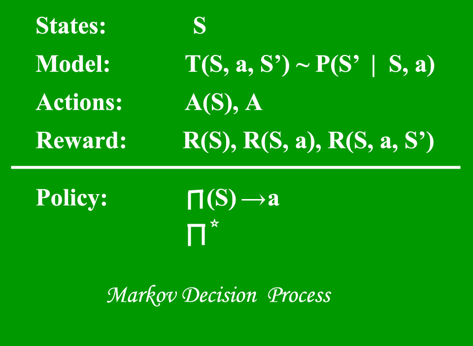
A Markov Decision Process (MDP) model contains:
A set of possible world states S.
A set of Models.
A set of possible actions A.
A real valued reward function R(s,a).
A policy the solution of Markov Decision Process.
What is a State?
A State is a set of tokens that represent every state that the agent can be in.
What is a Model?
A Model (sometimes called Transition Model) gives an action’s effect in a state. In particular, T(S, a, S’) defines a transition T where being in state S and taking an action ‘a’ takes us to state S’ (S and S’ may be same). For stochastic actions (noisy, non-deterministic) we also define a probability P(S’|S,a) which represents the probability of reaching a state S’ if action ‘a’ is taken in state S. Note Markov property states that the effects of an action taken in a state depend only on that state and not on the prior history.
What is Actions?
An Action A is set of all possible actions. A(s) defines the set of actions that can be taken being in state S.
What is a Reward?
A Reward is a real-valued reward function. R(s) indicates the reward for simply being in the state S. R(S,a) indicates the reward for being in a state S and taking an action ‘a’. R(S,a,S’) indicates the reward for being in a state S, taking an action ‘a’ and ending up in a state S’.
What is a Policy?
A Policy is a solution to the Markov Decision Process. A policy is a mapping from S to a. It indicates the action ‘a’ to be taken while in state S.
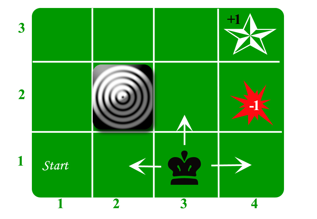
Let us take the example of a grid world:
An agent lives in the grid. The above example is a 3*4 grid. The grid has a START state(grid no 1,1). The purpose of the agent is to wander around the grid to finally reach the Blue Diamond (grid no 4,3). Under all circumstances, the agent should avoid the Fire grid (orange color, grid no 4,2). Also the grid no 2,2 is a blocked grid, it acts like a wall hence the agent cannot enter it.
The agent can take any one of these actions: UP, DOWN, LEFT, RIGHT
Walls block the agent path, i.e., if there is a wall in the direction the agent would have taken, the agent stays in the same place. So for example, if the agent says LEFT in the START grid he would stay put in the START grid.
First Aim: To find the shortest sequence getting from START to the Diamond. Two such sequences can be found:
RIGHT RIGHT UP UP RIGHT
UP UP RIGHT RIGHT RIGHT
Let us take the second one (UP UP RIGHT RIGHT RIGHT) for the subsequent discussion.
The move is now noisy. 80% of the time the intended action works correctly. 20% of the time the action agent takes causes it to move at right angles. For example, if the agent says UP the probability of going UP is 0.8 whereas the probability of going LEFT is 0.1 and probability of going RIGHT is 0.1 (since LEFT and RIGHT is right angles to UP).
The agent receives rewards each time step:-
Small reward each step (can be negative when can also be term as punishment, in the above example entering the Fire can have a reward of -1).
Big rewards come at the end (good or bad).
The goal is to Maximize sum of rewards.